Quantum walk

2022 Feb 23 in NTHU

Outline

1. Basic concepts of Quantum walk
2. Power of Quantum walk
3. Meet Physics

• Reference
  • Basic concepts
  • The Power of Quantum walk
  • Meet Physics
• Basic concepts
  • example
  • Structure
  • Infinite Lattices
    • The Fourier transform
    • eigen-problem of evolution operator
    • Analytic Solution
• Power of Quantum walk
  • Spatial search ~ modified evolution operator
  • complexity analysis ~ $b=0$">Case $B=0$
  • example 2D lattice

1. Reference

1.1.1. Basic concepts

1. Quantum Walks and Search Algorithms 2013 Renato Portugal
2. Quantum Walks and Quantum Computation 2013 Katharine Elizabeth Barr

1.1.2. The Power of Quantum walk

Quantum Walk Search

• Spatial search by quantum walk 2004 Andrew M. Childs
• Spatial search by quantum walk is optimal for almost all graphs 2015 arXiv:1508.01327

• A Unified Framework of Quantum Walk Search 2019

  Universal computation

• Universal computation by quantum walk 2009

1.1.3. Meet Physics

Topological phase

• Takuya Kitagawa

  1. Exploring Topological Phases With Quantum Walks 2010 arxiv.1003.1729
  2. Topological phenomena in quantum walks; elementary introduction to the physics of topological phases arXiv:1112.1882
  3. Observation of topologically protected bound states in photonic quantum walks 2012
     • Experimental

  spin glass

• Finding spin glass ground states using quantum walks 2019 arxiv.1903.05003

2. Basic concepts

2.1. example

The Hilbert space of the system is $H = H _{C} \otimes H _{P}$ where

• $H _{C}$ is the two-dimensional Hilbert space associated with the "coin," whose computational basis is $\{|0\rangle,|1\rangle\}$. We can now define the "coin" as any unitary matrix $C$ with dimension 2 , which acts on vectors in Hilbert space $H _{C} . C$ is called coin operator.
• the position of the walker is described by $|n\rangle$

The shift from $|n\rangle$ to $|n+1\rangle$ or $|n-1\rangle$ must be described by a unitary operator, called the shift operator $S$. It acts as follows: $\begin{array}{l} S|0\rangle|n\rangle=|0\rangle|n+1\rangle \\ S|1\rangle|n\rangle=|1\rangle|n-1\rangle \end{array}$ If we know the action of $S$ on the computational basis of $H$, we have a complete description of this linear operator, and we obtain $S=|0\rangle \langle 0 |\otimes \sum_{n=-\infty}^{\infty} | n+1 \rangle\langle n|+| 1\rangle \langle 1|\otimes \sum_{n=-\infty}^{\infty}| n-1\rangle\langle n| .$ Consider the particle initially located at the origin $|n=0\rangle$ and the coin state with spin up $|0\rangle$, that is, $|\psi(0)\rangle=|0\rangle|n=0\rangle$ where

• $|\psi(0)\rangle$ denotes the state of the quantum walk at $t=0$ and $|\psi(t)\rangle$ denotes the state at time $t$.

The most used coin is the Hadamard operator $H=\frac{1}{\sqrt{2}}\left[\begin{array}{cc} 1 & 1 \\ 1 & -1 \end{array}\right]$ One step consists of applying $H$ to the coin state followed by the shift operator $S$, in the following way: $\begin{aligned} |0\rangle \otimes|0\rangle & \stackrel{H \otimes I}{\longrightarrow} \frac{|0\rangle+|1\rangle}{\sqrt{2}} \otimes|0\rangle \\ & \stackrel{S}{\longrightarrow} \frac{1}{\sqrt{2}}(|0\rangle \otimes|1\rangle+|1\rangle \otimes|-1\rangle) . \end{aligned}$ After the first step, the position of the particle is a superposition of $n=1$ and $n=-1$.

The quantum walk dynamics are driven by the unitary operator $U=S(H \otimes I)$ with no intermediary measurements. One step consists in applying $U$ one time, which is equivalent to applying the coin operator followed by the shift operator.

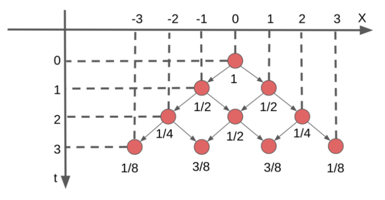
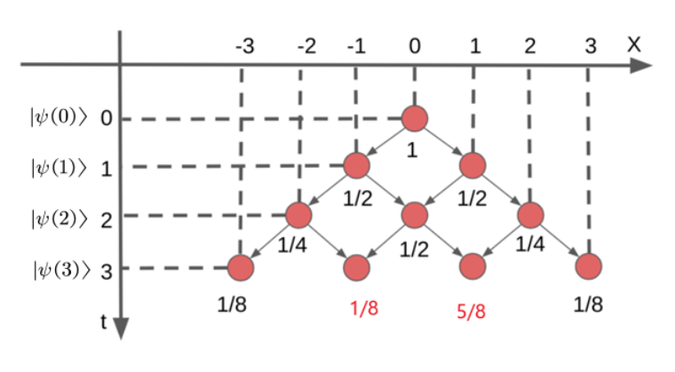
In the next step, we apply $U$ again without measurements. After $t$ steps, the state of the quantum walk is given by $|\psi(t)\rangle=U^{t}|\psi(0)\rangle$ The steps $\begin{aligned} |\psi(0)\rangle=&|0\rangle|n=0\rangle \\ |\psi(1)\rangle=&U^{1}|\psi(0)\rangle\\ =&\frac{1}{\sqrt{2}}(|1\rangle|-1\rangle+|0\rangle|1\rangle) \\ |\psi(2)\rangle=&U^{2}|\psi(0)\rangle\\ =&\frac{1}{2}(-|1\rangle|-2\rangle+(|0\rangle+|1\rangle)|0\rangle+|0\rangle|2\rangle)\\ |\psi(3)\rangle=&U^{3}|\psi(0)\rangle\\ =&\frac{1}{2 \sqrt{2}}(|1\rangle|-3\rangle-|0\rangle|-1\rangle+(2|0\rangle+|1\rangle)|1\rangle+|0\rangle|3\rangle) \end{aligned}$ We have used an unbiased coin, but the state $|\psi(3)\rangle$ is not symmetric

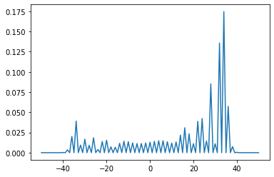
numerical calculate for large steps

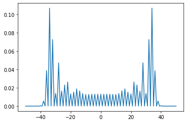
the probability distribution corresponding to the walker's position

change the initial condition $|\psi(0)\rangle=|0\rangle|n=0\rangle \longrightarrow |\psi(0)\rangle=\frac{|0\rangle- i |1\rangle}{\sqrt{2}}|n=0\rangle$ the state become symmetric

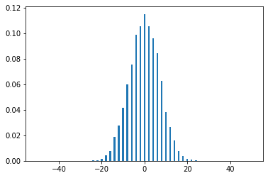
compare to classical random walk (Binomial distribution)

If $n$ is large enough, a reasonable approximation to $B(n, p)$ is given by the normal distribution $N (n p, n p(1-p))$ Standard deviation of

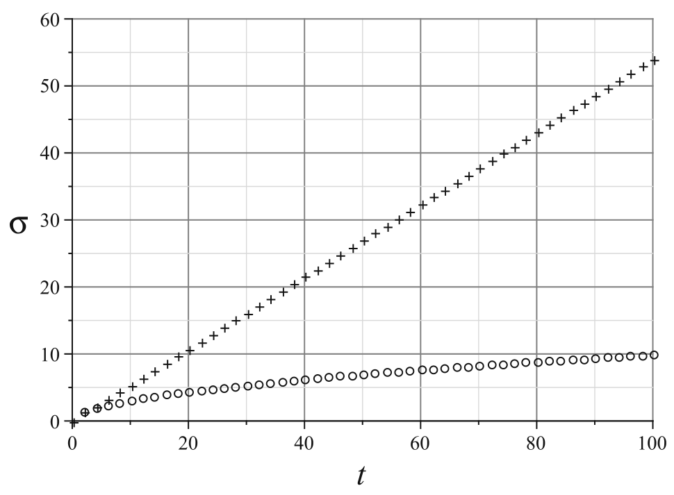
• the quantum walk (crosses) $\sigma(t)=0.54 t \propto t$
• the classical random walk (circles) $\sigma(t)=\sqrt{t}$

2.2. Structure

1. Finite Two-Dimensional Lattices
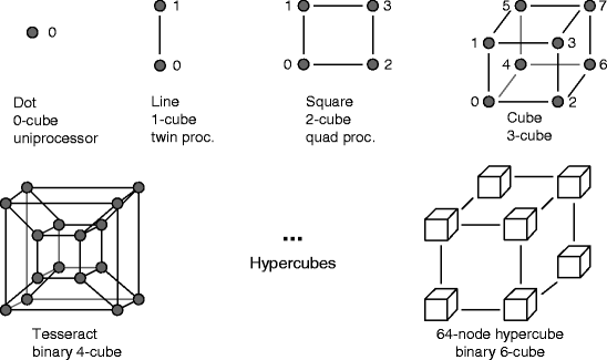
2. Hypercubes
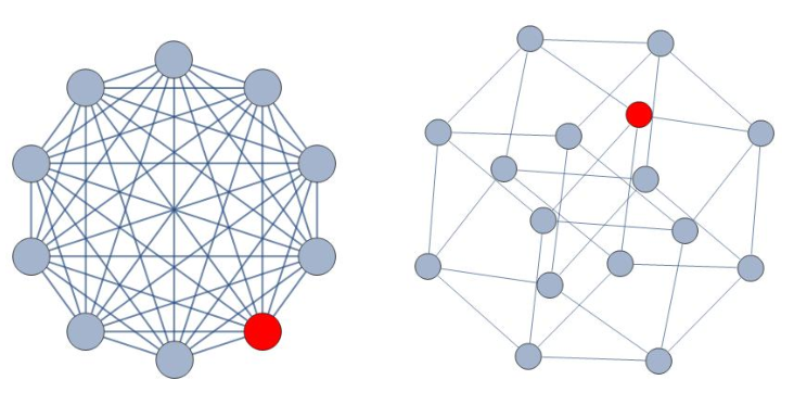
3. Graphs
   • Regular
   • Arbitrary

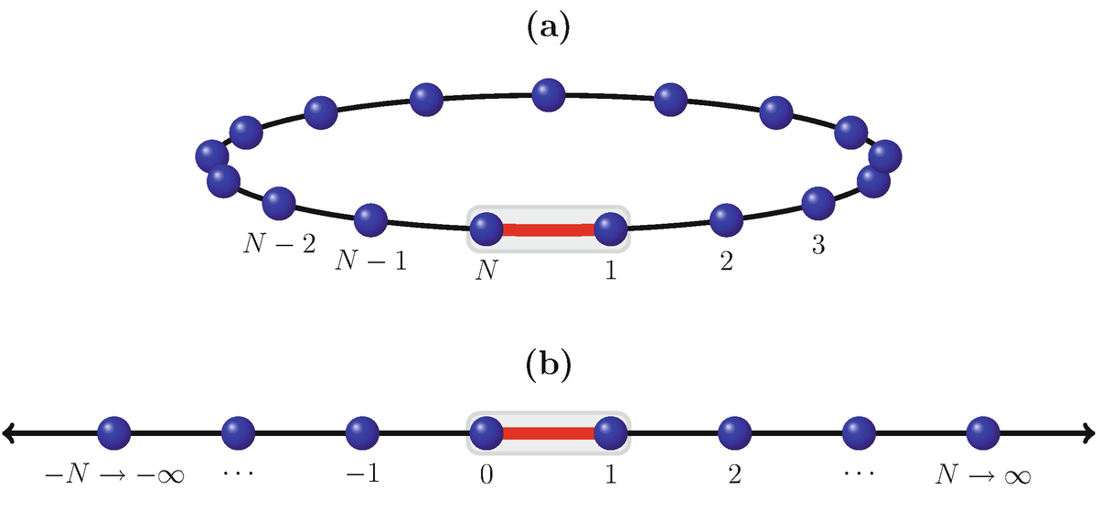
1. Coined Walks with Cyclic Boundary Conditions

2.3. Infinite Lattices

The full Hilbert space associated with the quantum walk $H _{C} \otimes H _{P}$ where

• computational basis is $\{|j, x\rangle: j \in\{0,1\}: x \in Z \}$

The state of the walker at time $t$ is described by $|\Psi(t)\rangle=\sum_{j=0}^{1} \sum_{x=-\infty}^{\infty} \psi_{j, x}(t)|j, x\rangle$ where

• the coefficients $\psi_{j, x}(t)$ are complex functions, called probability amplitudes,
• the probability distribution of a position measurement at the time step $t$

$p_{x}(t)=\left|\psi_{0, x}(t)\right|^{2}+\left|\psi_{1, x}(t)\right|^{2}$

The shift operator is $S=\sum_{j=0}^{1} \sum_{x=-\infty}^{\infty}\left|j, x+(-1)^{j}\right\rangle\langle j, x|$ Let us use the Hadamard coin $H=\frac{1}{\sqrt{2}}\left[\begin{array}{cc} 1 & 1 \\ 1 & -1 \end{array}\right]$ Applying the evolution operator of the coined model $U=S(H \otimes I)$ to state $|\Psi(t)\rangle$, we obtain $\begin{aligned} |\Psi(t+1)\rangle &=\sum_{x=-\infty}^{\infty} S\left(\psi_{0, x}(t) H|0\rangle|x\rangle+\psi_{1, x}(t) H|1\rangle|x\rangle\right) \\ &=\sum_{x=-\infty}^{\infty} \frac{\psi_{0, x}(t)+\psi_{1, x}(t)}{\sqrt{2}} S|0\rangle|x\rangle+\frac{\psi_{0, x}(t)-\psi_{1, x}(t)}{\sqrt{2}} S|1\rangle|x\rangle \\ &=\sum_{x=-\infty}^{\infty} \frac{\psi_{0, x}(t)+\psi_{1, x}(t)}{\sqrt{2}}|0\rangle|x+1\rangle \\ &\qquad+\frac{\psi_{0, x}(t)-\psi_{1, x}(t)}{\sqrt{2}}|1\rangle|x-1\rangle \end{aligned}$ corresponding coefficients on the right-hand side to obtain the walker's evolution equations $\begin{array}{l} \psi_{0, x}(t+1)=\frac{\psi_{0, x-1}(t)+\psi_{1, x-1}(t)}{\sqrt{2}} \\ \psi_{1, x}(t+1)=\frac{\psi_{0, x+1}(t)-\psi_{1, x+1}(t)}{\sqrt{2}} \end{array}$

2.3.1. The Fourier transform

The Fourier transform of a discrete function $f: Z \rightarrow C$ is a continuous function $\tilde{f}:[-\pi, \pi] \rightarrow C$ defined by $\tilde{f}(k)=\sum_{x=-\infty}^{\infty} e ^{- i k x} f(x)$ The Fourier transform of the coefficients $\psi_{j, x}(t)$ is $\widetilde{\psi}_{j}(k, t)=\sum_{x=-\infty}^{\infty} e ^{- i k x} \psi_{j, x}(t)$ There is another way to use the Fourier transform. $|\tilde{k}\rangle=\lim _{L \rightarrow \infty} \frac{1}{\sqrt{2 L+1}} \sum_{x=-L}^{L} e ^{ i k x}|x\rangle$ Fourier transform defines a new orthonormal basis $\{|j\rangle|\tilde{k}\rangle: j \in\{0,1\},-\pi \leq k \leq \pi\}$ called (extended) Fourier basis. In this basis, we can express the state of the quantum walk as $|\Psi(t)\rangle=\sum_{j=0}^{1} \int_{-\pi}^{\pi} \widetilde{\psi}_{j}(k, t)|j\rangle|\tilde{k}\rangle \frac{ d k}{2 \pi}$ the action of the shift operator on the new basis, $\begin{aligned} S|j\rangle|\tilde{k}\rangle &=\sum_{x=-\infty}^{\infty} e ^{ i k x} S|j, x\rangle \\ &=\sum_{x=-\infty}^{\infty} e ^{ i k x}|j\rangle\left|x+(-1)^{j}\right\rangle \end{aligned}$ Renaming index $x$ so that $x^{\prime}=x+(-1)^{j}$, $\begin{aligned} S|j\rangle|\tilde{k}\rangle &=\sum_{x^{\prime}=-\infty}^{\infty} e ^{ i k\left(x^{\prime}-(-1)^{j}\right)}|j\rangle\left|x^{\prime}\right\rangle \\ &= e ^{- i k(-1)^{j}}|j\rangle|\tilde{k}\rangle . \end{aligned}$ The result shows that the action of the shift operator $S$ on a state of the Fourier basis only changes its phase,

• $|j\rangle|\tilde{k}\rangle$ is an eigenvector associated with the eigenvalue $e ^{- i k(-1)^{j}}$.

2.3.2. eigen-problem of evolution operator

The next task is to find the eigenvectors of the evolution operator $U$. If we diagonalize $U$, we will be able to find an analytic expression for the state of the quantum walk as a function of time.

Applying $U$ to vector $\left|j^{\prime}\right\rangle|\tilde{k}\rangle$

$\begin{aligned} U\left|j^{\prime}\right\rangle|{k}\rangle &=S\left(\sum_{j=0}^{1} H_{j, j^{\prime}}|j\rangle|\tilde{k}\rangle\right) \\ &=\sum_{j=0}^{1} e ^{- i k(-1)^{j}} H_{j, j^{\prime}}|j\rangle|\tilde{k}\rangle \end{aligned}$ The entries of $U$ in the Fourier basis are $\left\langle j, \tilde{k}|U| j^{\prime}, \tilde{k}^{\prime}\right\rangle= e ^{- i k(-1)^{j}} H_{j, j^{\prime}} \delta_{k, k^{\prime}} .$ For each $k$, we define operator $\widetilde{H}_{k}$, whose entries are $\widetilde{H}_{j, j^{\prime}}= e ^{- i k(-1)^{j}} H_{j, j^{\prime}}$ In the matrix form, we have $\begin{aligned} \tilde{H}_{k} &=\left[\begin{array}{cc} e ^{- i k} & 0 \\ 0 & e ^{ i k} \end{array}\right] \cdot H \\ &=\frac{1}{\sqrt{2}}\left[\begin{array}{ll} e ^{- i k} & e ^{- i k} \\ e ^{ i k} & - e ^{ i k} \end{array}\right] \end{aligned}$ The action of the shift operator $S$ has been absorbed by $\widetilde{H}_{k}$ when $U$ acts on $|j\rangle|\tilde{k}\rangle$. If $\left|\alpha_{k}\right\rangle$ is an eigenvector of $\widetilde{H}_{k}$ with eigenvalue $\alpha_{k}$, we have $\begin{aligned} U\left|\alpha_{k}\right\rangle|\tilde{k}\rangle &=\left(\widetilde{H}_{k}\left|\alpha_{k}\right\rangle\right)|\tilde{k}\rangle \\ &=\alpha_{k}\left|\alpha_{k}\right\rangle|\tilde{k}\rangle . \end{aligned}$ Therefore, $\left|\alpha_{k}\right\rangle|\tilde{k}\rangle$ is an eigenvector of $U$ associated with the eigenvalue $\alpha_{k}$.

This result shows that the diagonalization of the evolution operator reduces to the diagonalization of $\widetilde{H}_{k} .$

• $U$ acts on an infinite-dimensional Hilbert space,
• while $\widetilde{H}_{k}$ acts on a two-dimensional space.

The characteristic polynomial of $\widetilde{H}_{k}$ is $p_{\widetilde{H}_{k}}(\lambda)=\lambda^{2}+ i \sqrt{2} \lambda \sin k-1 .$ The eigenvalues are the solutions of $p_{\widetilde{H}_{k}}(\lambda)=0$, which are $\begin{aligned} \alpha_{k} &= e ^{- i \omega_{k}} \\ \beta_{k} &= e ^{ i \left(\pi+\omega_{k}\right)} \end{aligned}$ where $\omega_{k}$ is an angle in the interval $[-\pi / 2, \pi / 2]$ that satisfies the equation $\sin \omega_{k}=\frac{1}{\sqrt{2}} \sin k .$

The normalized eigenvectors are $\left|\alpha_{k}\right\rangle=\frac{1}{\sqrt{c^{-}}}\left[\begin{array}{c} e ^{- i k} \\ \sqrt{2} e ^{- i \omega_{k}}- e ^{- i k} \end{array}\right]$

$\left|\beta_{k}\right\rangle=\frac{1}{\sqrt{c^{+}}}\left[\begin{array}{c} e ^{- i k} \\ \left.-\sqrt{2} e ^{ i \omega_{k}}- e ^{- i k}\right. \end{array}\right]$

where $c^{\pm}=2\left(1+\cos ^{2} k\right) \pm 2 \cos k \sqrt{1+\cos ^{2} k}$ The spectral decomposition of $U$ is $U=\int_{-\pi}^{\pi}\left( e ^{- i \omega_{k}}\left|\alpha_{k}, \tilde{k}\right\rangle\left\langle\alpha_{k}, \tilde{k}\left|+ e ^{ i \left(\pi+\omega_{k}\right)}\right| \beta_{k}, \tilde{k}\right\rangle\left\langle\beta_{k}, \tilde{k}\right|\right) \frac{ d k}{2 \pi}$ The $t$ th power of $U$ is $U^{t}=\int_{-\pi}^{\pi}\left( e ^{- i \omega_{k} t}\left|\alpha_{k}, \tilde{k}\right\rangle\left\langle\alpha_{k}, \tilde{k}\left|+ e ^{ i \left(\pi+\omega_{k}\right) t}\right| \beta_{k}, \tilde{k}\right\rangle\left\langle\beta_{k}, \tilde{k}\right|\right) \frac{ d k}{2 \pi}$ because a function applied to $U$ is by definition applied directly to the eigenvalues when $U$ is written in its eigenbasis. In this case, the function is $f(x)=x^{t}$

2.3.3. Analytic Solution

Suppose that initially the walker is at the origin $x=0$ and the coin state is $|0\rangle$. The initial condition is $|\psi(0)\rangle=|0\rangle|x=0\rangle .$ we obtain $\begin{aligned} |\psi(t)\rangle=& U^{t}|\psi(0)\rangle \\ =& \int_{-\pi}^{\pi}\left( e ^{- i \omega_{k} t}\left|\alpha_{k}, \tilde{k}\right\rangle\left\langle\alpha_{k}, \tilde{k} \mid 0,0\right\rangle\right.\\ &\left.+ e ^{ i \left(\pi+\omega_{k}\right) t}\left|\beta_{k}, \tilde{k}\right\rangle\left\langle\beta_{k}, \tilde{k} \mid 0,0\right\rangle\right) \frac{ d k}{2 \pi} \end{aligned}$ Using $\left|\alpha_{k}\right\rangle=\frac{1}{\sqrt{c^{-}}}\left[\begin{array}{c} e ^{- i k} \\ \sqrt{2} e ^{- i \omega_{k}}- e ^{- i k}\end{array}\right]$, $\left|\beta_{k}\right\rangle=\frac{1}{\sqrt{c^{+}}}\left[\begin{array}{c} e ^{- i k} \\ -\sqrt{2} e ^{ i \omega_{k}}- e ^{- i k}\end{array}\right]$ we obtain $\begin{aligned} \left\langle\alpha_{k}, \tilde{k} \mid 0,0\right\rangle &=\frac{ e ^{ i k}}{\sqrt{c^{-}}} \\ \left\langle\beta_{k}, \tilde{k} \mid 0,0\right\rangle &=\frac{ e ^{ i k}}{\sqrt{c^{+}}} \end{aligned}$ Then, $|\psi(t)\rangle=\int_{-\pi}^{\pi}\left(\frac{ e ^{- i \left(\omega_{k} t-k\right)}}{\sqrt{c^{-}}}\left|\alpha_{k}\right\rangle+\frac{ e ^{ i \left(\pi+\omega_{k}\right) t+ i k}}{\sqrt{c^{+}}}\left|\beta_{k}\right\rangle\right)|\tilde{k}\rangle \frac{ d k}{2 \pi}$

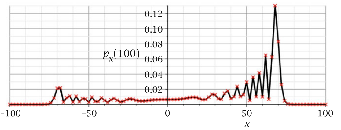
Probability distribution of the quantum walk on the line after 100 steps obtained from the analytic expressions $\begin{array}{l} \psi_{0, x}(t)=\int_{-\pi}^{\pi}\left(1+\frac{\cos k}{\sqrt{1+\cos ^{2} k}}\right) e ^{- i \left(\omega_{k} t-k x\right)} \frac{ d k}{2 \pi} \\ \psi_{1, x}(t)=\int_{-\pi}^{\pi} \frac{ e ^{ i k}}{\sqrt{1+\cos ^{2} k}} e ^{- i \left(\omega_{k} t-k x\right)} \frac{ d k}{2 \pi} \end{array}$

3. Power of Quantum walk

Spatial search

1. Spatial search by quantum walk 2004 Andrew M. Childs arXiv:quant-ph/0306054
2. Spatial search by quantum walk is optimal for almost all graphs 2015 arXiv:1508.01327

Universal computation

1. Universal computation by quantum walk 2009

3.1. Spatial search

the spatial search problem, which aims to find one or more marked points in a finite physical region that can be modeled by a graph

Consider a graph $\Gamma$, where

• $V(\Gamma)$ is the set of vertices
• $|V(\Gamma)|=N$.

Let $H ^{N}$ be the $N$-dimensional Hilbert space associated with the graph, that is, the computational basis of $H ^{N}$ is $\{|v\rangle: 0 \leq v \leq N-1\}$ Let $M$ be the set of marked vertices. Then, the unitary operator we need is $R=I-2 \sum_{v \in M}|v\rangle\langle v|$ The next step is to build an evolution operator $U$ associated with the graph.

modified evolution operator

The evolution operator $U^{\prime}$ of a quantum-walk-based search algorithm is $U^{\prime}=U R$ where

• $U^{\prime}$ is called modified evolution operator to distinguish from $U$.

• $U$ is the standard evolution operator of a quantum walk on the graph with no marked vertex

• $R$ is the unitary operator that inverts the sign of the marked vertex

In this context

• the walker starts at an initial state $|\psi(0)\rangle$
• and evolves driven by $U^{\prime}$
• that is, the walker's state after $t$ steps is $|\psi(t)\rangle=\left(U^{\prime}\right)^{t}|\psi(0)\rangle$.

eigenvalue and eigenvectors of the modified evolution operator $U^{\prime}$.

$U^{\prime}|\lambda\rangle=\exp ( i \lambda)|\lambda\rangle$ where

• Let $\exp \left( i \lambda_{1}\right), \ldots$, $\exp \left( i \lambda_{k}\right)$ be the eigenvalues $U^{\prime}$ such that $\lambda_{1}, \ldots, \lambda_{k} \in[-\pi, \pi] .$

1. Select the smallest positive element of the set $\left\{\lambda_{1}, \ldots, \lambda_{k}\right\}$. Let us call this smallest element by $\lambda$ and the unit eigenvector by $|\lambda\rangle$, that is $\langle\lambda \mid \lambda\rangle=1$.
2. Select the largest negative element of the set $\left\{\lambda_{1}, \ldots, \lambda_{k}\right\}$. Let us call this largest negative element by $\lambda^{\prime}$ and the unit eigenvector by $\left|\lambda^{\prime}\right\rangle$,

In most spatial search algorithms $\lambda^{\prime}=-\lambda$ vectors $|\lambda\rangle$ and $\left|\lambda^{\prime}\right\rangle$ are the only eigenvectors of $U^{\prime}$

1. f the graph on which the quantum walk takes place is simple enough, such as the complete graph, we can calculate $\lambda$ and $\lambda^{\prime}$ without much effort.
2. For an arbitrary graph, we describe a technique we call principal eigenvalue technique, which allows to find $\lambda$ and $\lambda^{\prime}$.

3.2. complexity analysis

The complexity analysis of the spatial search algorithm is based on two quantities:

• The running time $t_{ opt }$
• the success probability $p\left(t_{ opt }\right)$

The expression of the probability of finding the marked vertex 0 after $t$ steps is $p(t)=|\langle 0 \mid \psi(t)\rangle|^{2}$ Since $|\psi(t)\rangle=$ $\left(U^{\prime}\right)^{t}|\psi(0)\rangle$, we have $p(t)=\left|\left\langle 0\left|\left(U^{\prime}\right)^{t}\right| \psi(0)\right\rangle\right|^{2}$

The goal now is to determine the optimal number of steps $t_{\text {opt }}$, which is the one that maximizes $p(t)$.

The spectral decomposition of $U^{\prime}$ would be $U^{\prime}= e ^{ i \lambda}|\lambda\rangle\left\langle\lambda\left|+ e ^{ i \lambda^{\prime}}\right| \lambda^{\prime}\right\rangle\left\langle\lambda^{\prime}\right|+U_{\text {tiny }}$ where $U_{\text {tiny }}$ acts nontrivially only on the subspace orthogonal to the plane spanned by $\left\{|\lambda\rangle,\left|\lambda^{\prime}\right\rangle\right\}$. After raising the previous equation to power $t$ we obtain $\left(U^{\prime}\right)^{t}= e ^{ i \lambda t}|\lambda\rangle \langle\lambda|+ e ^{ i \lambda^{\prime} t} | \lambda^{\prime} \rangle\left\langle\lambda^{\prime}\right|+U_{\text {tiny }}^{t}$ the probability $p(t)=\left| e ^{ i \lambda t}\langle 0 \mid \lambda\rangle\langle\lambda \mid \psi(0)\rangle+ e ^{ i \lambda^{\prime} t}\left\langle 0 \mid \lambda^{\prime}\right\rangle\left\langle\lambda^{\prime} \mid \psi(0)\right\rangle+\epsilon\right|^{2}$ where

• $\epsilon=\left\langle 0\left|U_{\text {tiny }}^{t}\right| \psi(0)\right\rangle$ From now on we will disregard $\epsilon$

We need to find $\lambda, \lambda^{\prime}$, the inner products $\langle 0 \mid \lambda\rangle,\langle\lambda \mid \psi(0)\rangle$, and their primed versions.

We skip some procedures and directly get the equation $\begin{aligned} \sum_{\phi_{k}=0}\left|\left\langle 0 \mid \psi_{k}\right\rangle\right|^{2} \frac{\sin \lambda}{1-\cos \lambda}+\sum_{\phi_{k} \neq 0}\left|\left\langle 0 \mid \psi_{k}\right\rangle\right|^{2} \frac{\sin \left(\lambda-\phi_{k}\right)}{1-\cos \left(\lambda-\phi_{k}\right)}=&0\\ A-B \lambda-C \lambda^{2}=&O\left(\lambda^{3}\right) \end{aligned}$ where $\begin{aligned} A=&2 \sum_{\phi_{k}=0}\left|\left\langle 0 \mid \psi_{k}\right\rangle\right|^{2} \\ B=&\sum_{\phi_{k} \neq 0} \frac{\left|\left\langle 0 \mid \psi_{k}\right\rangle\right|^{2} \sin \phi_{k}}{1-\cos \phi_{k}} \\ C=&\sum_{\phi_{k} \neq 0} \frac{\left|\left\langle 0 \mid \psi_{k}\right\rangle\right|^{2}}{1-\cos \phi_{k}} \end{aligned}$ We can find $\lambda$ by solving $A-B \lambda-C \lambda^{2}=O\left(\lambda^{3}\right)$ Our goal now is to find $\langle 0 \mid \lambda\rangle$. Making a sandwich with $|\lambda\rangle$ on both sides of $I=\sum_{k}\left|\psi_{k}\right\rangle\left\langle\psi_{k}\right|$, we obtain $1=\sum_{k}\left|\left\langle\psi_{k} \mid \lambda\right\rangle\right|^{2}$. Using $\left\langle\psi_{k} \mid \lambda\right\rangle=\frac{2\langle 0 \mid \lambda\rangle\left\langle\psi_{k} \mid 0\right\rangle}{1- e ^{ i \left(\lambda-\phi_{k}\right)}}$, we obtain $\frac{1}{|\langle 0 \mid \lambda\rangle|^{2}}=\sum_{k} \frac{4\left|\left\langle 0 \mid \psi_{k}\right\rangle\right|^{2}}{\mid 1- e ^{\left. i \left(\lambda-\phi_{k}\right)\right|^{2}}}$ Without loss of generality, we may assume that $\langle 0 \mid \lambda\rangle$ is a positive real number. In fact, if $\langle 0 \mid \lambda\rangle=a e ^{ i b}$, where $a$ and $b$ are real numbers and $a$ is positive, we redefine $|\lambda\rangle$ as $e ^{-1 b}|\lambda\rangle$. We are allowed to do this redefinition because a multiple of an eigenvector is also an eigenvector and in this case the norm of the eigenvector does not change. After this redefinition and using that $\left|1- e ^{ i a}\right|^{2}=2(1-\cos a)$, we obtain $\langle 0 \mid \lambda\rangle=\frac{|\lambda|}{\sqrt{2} \sqrt{A+C \lambda^{2}}}+O(\lambda)$ Our goal now is to find $\langle\lambda \mid \psi(0)\rangle$. We choose $|\psi(0)\rangle$ as an eigenvector of $U$ with eigenvalue $1 .^{3}$ In this case, $\left\langle\psi_{k} \mid \lambda\right\rangle=\frac{2\langle 0 \mid \lambda\rangle\left\langle\psi_{k} \mid 0\right\rangle}{1- e ^{ i \left(\lambda-\phi_{k}\right)}}$ we can replace in $\left|\psi_{k}\right\rangle$ by $|\psi(0)\rangle$ and $\phi_{k}$ by 0 to obtain $\langle\psi(0) \mid \lambda\rangle=\frac{2\langle 0 \mid \lambda\rangle\langle\psi(0) \mid 0\rangle}{1- e ^{ i \lambda}}$ Using $2 /\left(1- e ^{ i \lambda}\right)=1+ i \sin \lambda /(1-\cos \lambda)$, we obtain $\langle\psi(0) \mid \lambda\rangle=\langle\psi(0) \mid 0\rangle\langle 0 \mid \lambda\rangle\left(1+\frac{i \sin \lambda}{1-\cos \lambda}\right)$

Case $B=0$

If the eigenvalues of $U$ come in complex-conjugate pairs, that is, both $e ^{ i \phi_{k}}$ and $e ^{- i \phi_{k}}$ are eigenvalues, and the corresponding values of $\left|\left\langle 0 \mid \psi_{k}\right\rangle\right|$ are equal, for instance, when the eigenvector associated with $e ^{- i \phi_{k}}$ is the complex conjugate of the eigenvector associated with $e ^{ i \phi_{k}}, B$ is zero

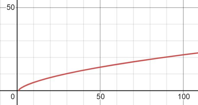
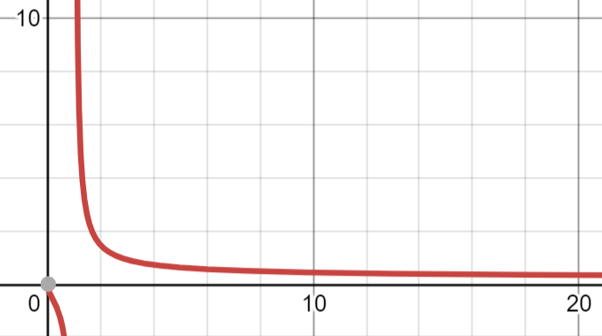
When $B=0$, Eq. $A-B \lambda-C \lambda^{2}=O\left(\lambda^{3}\right)$ reduces to $\lambda=-\lambda^{\prime}=\frac{\sqrt{A}}{\sqrt{C}}$ Equation $\langle 0 \mid \lambda\rangle=\frac{|\lambda|}{\sqrt{2} \sqrt{A+C \lambda^{2}}}+O(\lambda)$ reduces to $\langle 0 \mid \lambda\rangle=\left\langle 0 \mid \lambda^{\prime}\right\rangle=\frac{1}{2 \sqrt{C}}$ and Eq. $\langle\psi(0) \mid \lambda\rangle=\langle\psi(0) \mid 0\rangle\langle 0 \mid \lambda\rangle\left(1+\frac{i \sin \lambda}{1-\cos \lambda}\right)$ reduces to $\langle\psi(0) \mid \lambda\rangle=\left\langle\lambda^{\prime} \mid \psi(0)\right\rangle=\langle\psi(0) \mid 0\rangle\left(\frac{1}{2 \sqrt{C}}+\frac{ i }{\sqrt{A}}\right) .$ Substituting those results into $\begin{aligned} p(t)=&\left| e ^{ i \lambda t}\langle 0 \mid \lambda\rangle\langle\lambda \mid \psi(0)\rangle+ e ^{ i \lambda^{\prime} t}\left\langle 0 \mid \lambda^{\prime}\right\rangle\left\langle\lambda^{\prime} \mid \psi(0)\right\rangle+\epsilon\right|^{2}\\ =&\frac{|\langle 0 \mid \psi(0)\rangle|^{2}}{A C} \sin ^{2} \lambda t \end{aligned}$ The running time is the optimal $t$, which is $t_{ opt }=\left\lfloor\frac{\pi}{2 \lambda}\right\rfloor$ and the asymptotic success probability is $p_{\text {succ }}=\frac{|\langle 0 \mid \psi(0)\rangle|^{2}}{A C}$ An important case is when $|\psi(0)\rangle$ is the diagonal state and the only (modulo a multiplicative constant) $(+1)$-eigenvector of $U$ that has nonzero overlap with $|0\rangle$. In this case, $A=2|\langle 0 \mid \psi(0)\rangle|^{2}=2 / N$ and the running time is $t_{ opt }=\left\lfloor\frac{\pi \sqrt{N C}}{2 \sqrt{2}}\right\rfloor$ and the success probability is $p_{\text {succ }}=\frac{1}{2 C}$ In this case, the complexity of the algorithm is determined by $C$. For the twodimensional lattice, $C=O(\ln N)$. The running time is $O(\sqrt{N \ln N})$ and the success probability is $O(1 / \ln N)$. The best scenario we can hope for is $C=O(1)$, which achieves the Grover lower bound, that is, the running time is $t_{\text {opt }}=O(\sqrt{N})$ with constant success probability.

3.3. example 2D lattice

in the $\sqrt{N} \times \sqrt{N}$ square lattice with periodic boundary conditions. The evolution operator of a coined quantum walk with no marked vertex is $U=S(G \otimes I)$ where $G$ is the Grover coin and $S$ is the flip-flop shift operator. The details are described in Sect. $6.2$ on p. 98 .

A search algorithm on the lattice is driven by the modified evolution operator $U^{\prime}=U R^{\prime}$ where $R^{\prime}=I-2\left|0^{\prime}\right\rangle\left\langle 0^{\prime}\right|$ with $\left|0^{\prime}\right\rangle=\left| D _{C}\right\rangle|0,0\rangle$ where $\left| D _{C}\right\rangle$ is the diagonal state of the coined space and $\left| D _{P}\right\rangle$ is the diagonal state of the position space. This state can be generated by $O(\sqrt{N})$ steps

We list the eigenvectors that have nonzero overlap with $\left|0^{\prime}\right\rangle$. The only eigenvector with eigenvalue 1 is $\left|\nu_{0,0}^{1 a}\right\rangle|\tilde{0}, \tilde{0}\rangle$ which is equal to the initial condition $|\psi(0)\rangle$. The remaining eigenvectors are $\left|\nu_{k \ell}^{\pm \theta}\right\rangle|\tilde{k}, \tilde{\ell}\rangle$ for $0 \leq k, l<\sqrt{N}$ and $(k, l) \neq(0,0)$, where $\left|\nu_{k \ell}^{\pm \theta}\right\rangle=\frac{ i }{2 \sqrt{2} \sin \theta_{k \ell}}\left[\begin{array}{l} e ^{ Fi \theta_{k \ell}}-\omega^{k} \\ e ^{\mp i \theta_{k \ell}}-\omega^{-k} \\ e ^{ Fi \theta_{k \ell}}-\omega^{\ell} \\ e ^{ Fi \theta_{k \ell}}-\omega^{-\ell} \end{array}\right]$ which have eigenvalues $e ^{\pm i \theta_{k \ell}}$, where $\theta_{k \ell}$ are given by $\cos \theta_{k \ell}=\frac{1}{2}\left(\cos \frac{2 \pi k}{\sqrt{N}}+\cos \frac{2 \pi \ell}{\sqrt{N}}\right)$ and $\omega= e ^{\frac{2 \pi i}{\sqrt{N}}}$.

Vector $|\tilde{k}, \tilde{\ell}\rangle$ is the Fourier transform given by Eq. $|\tilde{k}, \tilde{\ell}\rangle=\frac{1}{\sqrt{N}} \sum_{x, y=0}^{\sqrt{N}-1} \omega^{x k+y \ell}|x, y\rangle$. Note that the eigenvalues and eigenvectors of $U$ come in complex-conjugate pairs, Note that the eigenvalues and eigenvectors of $U$ come in complex-conjugate pairs, two-dimensional lattice, $\phi_{k} \rightarrow \theta_{k \ell},\left|\psi_{k}\right\rangle \rightarrow\left|\nu_{k \ell}^{\pm \theta}\right\rangle|{k}, \tilde{\ell}\rangle, \sum_{k} \rightarrow \sum_{k \ell}$, and using that $\left\langle 0^{\prime}\right|=\left\langle D _{C}\right|\langle 0,0|$, we obtain $\begin{aligned} A=&\frac{2}{N}, \\ B=&0, \\ C=&\frac{1}{N} \sum_{k, \ell=0 \atop(k, \ell) \neq(0,0)}^{\sqrt{N}-1} \frac{1}{1-\frac{1}{2}\left(\cos \frac{2 \pi k}{\sqrt{N}}+\cos \frac{2 \pi \ell}{\sqrt{N}}\right)} \\ =&c \ln N+O(1) \end{aligned}$ where $c$ is a number bounded by $2 / \pi^{2} \leq c \leq 1$. Numerical calculations show that $c=0.33$ approximately. Since $B=0$, the probability of finding the marked vertex as a function of the number of steps is given by Eq. $p(t)=\frac{|\langle 0 \mid \psi(0)\rangle|^{2}}{A C} \sin ^{2} \lambda t$. For the two-dimensional square lattice with odd $\sqrt{N}$,
$p(t)=\frac{1}{2 c \ln N} \sin ^{2}\left(\frac{\sqrt{2} t}{\sqrt{c} \sqrt{N \ln N}}\right) .$ The running time is $t_{ opt }=\left\lfloor\frac{\pi \sqrt{c} \sqrt{N \ln N}}{2 \sqrt{2}}\right\rfloor$ and the success probability is $p_{\text {succ }}=\frac{1}{2 c \ln N}+O\left(N^{-1}\right) .$

1. Note that the running time is good enough because it is the square root of the classical hitting time.
2. On the other hand, the success probability seems disappointing because it tends to zero when $N$ increases. Since it goes to zero logarithmically in terms of $N$, the situation is not too bad and can be saved.